This article explores the hidden structures that emerge when materials break apart, revealing unexpected connections between natural processes, mathematics, and art. In particular, it examines Alberto Burri’s Grande cretto nero, whose fracturing evokes hyperbolic geometry reminiscent of Poincaré’s models and Escher’s tessellations. Through this interdisciplinary journey, the article shows how close attention to seemingly trivial phenomena can inspire profound insights across science and art.
Imagine walking through a forest. At first everything seems ordinary—the fallen leaves on the ground, the cracks in the drying mud along the path, the songs of birds overhead. But if you pause for a moment and look more closely, your perception may suddenly shift: held against the sun, a leaf reveals a delicate network of veins, the cracks, once random, now divide space into polygons and the bird calls fall into a structured rhythm. What seemed trivial a moment ago now appears deeply ordered… and somehow, beautiful.
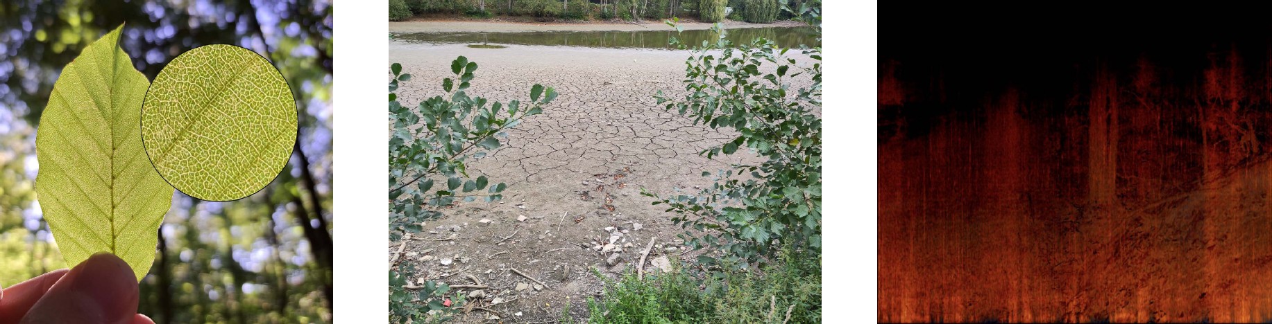
But how do such moments emerge? And why should they matter to us, apart from leaving us momentarily amazed? Part of the answer may lie in a remarkable human ability: the capacity to hold our breath and intentionally focus on what at first appears as ordinary.
These encounters with nature, these tiny moments, spark our curiosity and set our minds in motion. Each observation begins with something common yet carries the seed of a story: a moment when someone noticed a regularity, asked a question, and sought an explanation. What begins as simple curiosity can grow into structure, classification, and, in time, theory.
In this sense, the ability to perceive order within apparent randomness lies at the root of science, and of mathematics itself.
Reading the cracks
Patterns are universal. They can be found in every object and every material, in plants and animals alike: from stripes in the fur of a tiger, structural colors in butterfly wings, or the fractal growth forms of stony corals. And even when things break apart, decompose and decay, physical laws are at play, guiding the process toward some structured outcome.
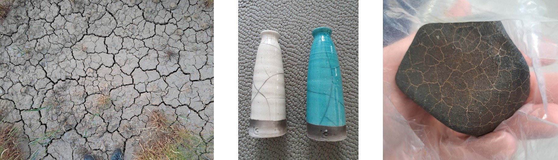
Among these diverse expressions of order, this article turns to one phenomenon in particular: the formation of cracks. When a material gives way under stress, the release of tension inscribes itself as a network of fissures. Such networks are visible in drying mud, in the glaze of ceramics, or even in the fusion crust of meteorites. They are at once destructive and generative, producing geometries of striking regularity.
Locally, a single crack may appear structureless and random, but the situation becomes far more interesting when two or more cracks are at play. Imagine an old concrete pavement with two cracks approaching each other from opposite directions. At first, it seems as if the cracks try to avoid and turn around one other, only to meet moments later, at nearly right angles. This pattern repeats across countless materials and situations. But why? How does one crack influence the path of another? How do they “communicate”?
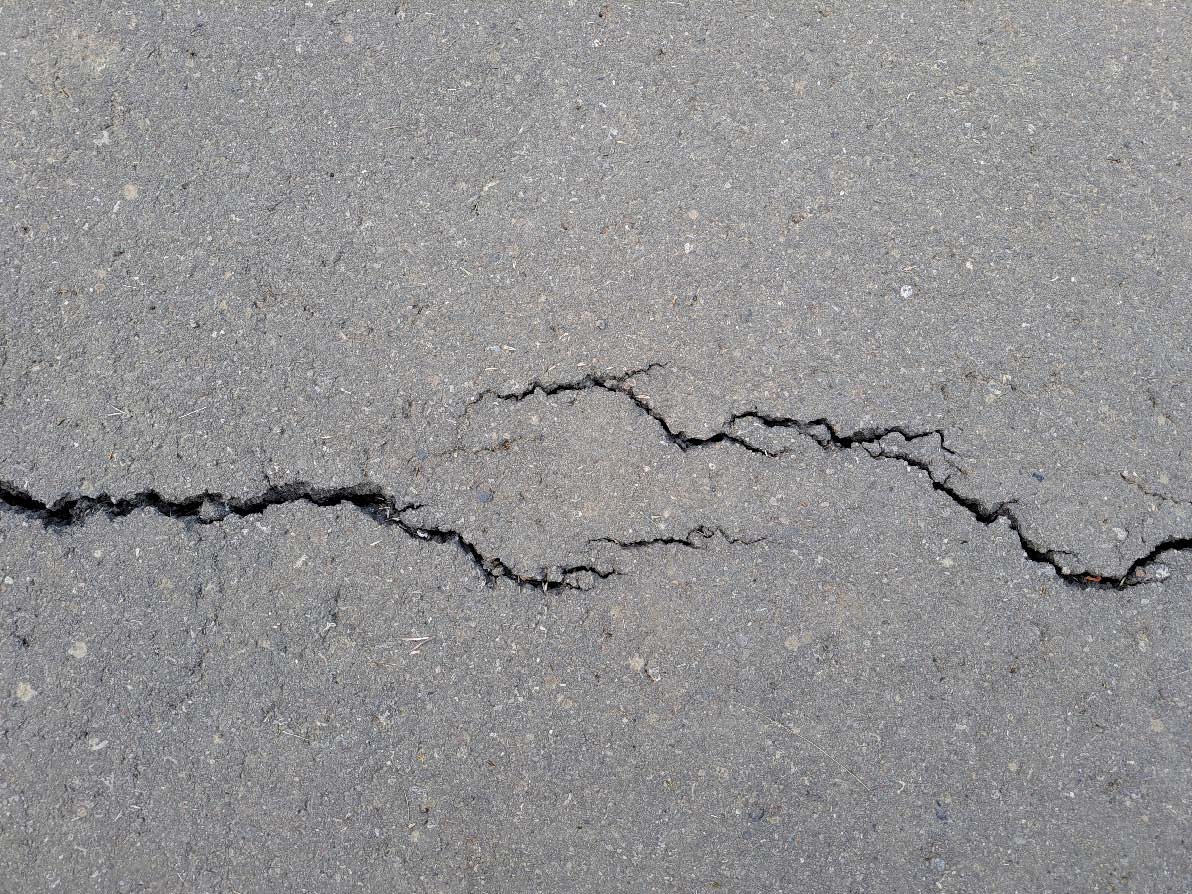
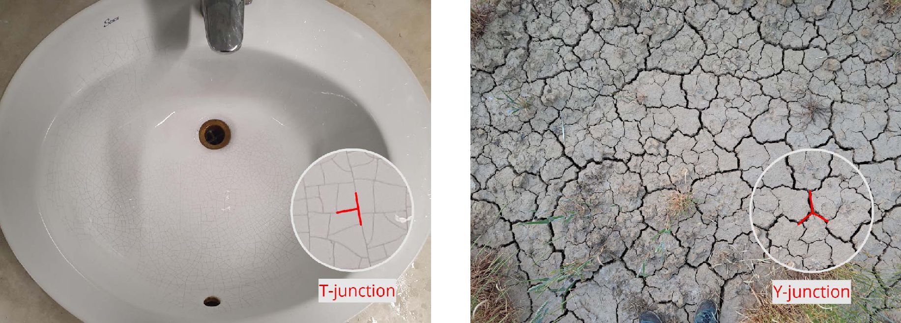
The answer lies in the material itself. As a crack propagates, it releases tension along its path, leaving the remaining stress oriented perpendicular to the crack. When a second crack approaches, it tends to grow in the direction that maximizes the release of this residual stress. This naturally leads the cracks to meet at angles of roughly 90°, forming what is typically called a T-junction.
The story becomes more complex when cracks repeatedly heal and break again, as for instance in mud subjected to cycles of wetting and drying. In such cases, T-junctions can evolve into so-called Y-junctions, where the cracks meet at angles of about 120°, distributing stress evenly in three directions. Thus, the geometry of crack junctions depends strongly on the physical process behind the cracking.
A striking example with profound implications comes from planet Mars, where NASA’s Curiosity rover discovered networks of hexagonal mud cracks in Gale Crater. Captured in 2021, these patterns provide the first direct evidence of sustained wet-dry cycling on the planet [3 W. Rapin, G. Dromart, B. C. Clark, J., Schieber, E. S. Kite, L. C. Kah, L. M. Thompson, O. Gasnault, J. Lasue, P.-Y. Meslin, P. I. Gasda and N. L. Lanza, Sustained wet–dry cycling on early Mars. Nature 620, 299–302 (2023) ]. Unlike the sharp T-junctions produced in single drying events, the hexagons formed only after repeated rehydration gradually softened the angles into Y-junctions. Such cyclic wetting and drying is particularly significant, as it is thought to create the conditions necessary for the chemical steps that precede life. Thus, these Martian cracks not only record ancient climate but also hint at environments once capable of supporting the chemistry of life’s origins.
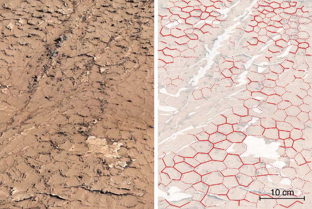
NASA / JPL-Caltech / MSSS / IRAP
The hidden geometry of things breaking apart
Apart from the physical processes that govern how cracks form, under the right conditions, their networks surprisingly follow purely mathematical rules, grounded in simple combinatorial arguments.
Imagine taking a blank sheet of paper and drawing randomly straight lines across it. The lines divide the sheet into a mosaic of regions. If you count the number of vertices of each region and then take the average, you will always find the result close to four.
To see this, let be the number of vertices in a given region. When a new line divides this region into two, let and denote the numbers of vertices in the resulting regions.
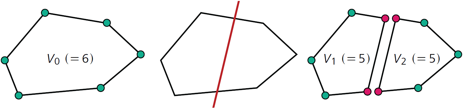
Splitting the region into two, the average number of vertices is given by
or equivalently .
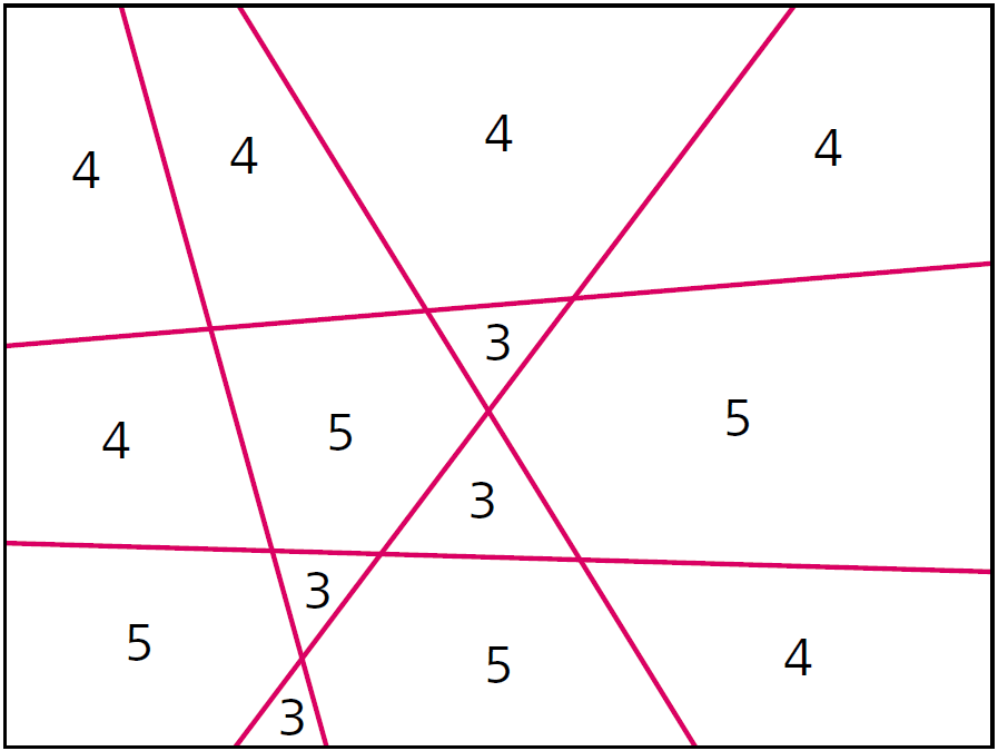
Each time the process is repeated, the distance to 4 is cut in half so that approaches 4.
This very simple and purely mathematical reasoning applies to real world networks of cracks made of straight lines. A simple example of this are broken ice plates.
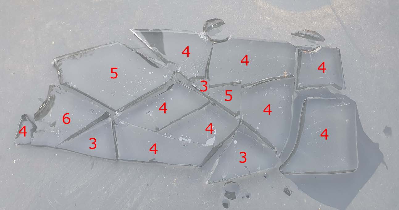
In a widely discussed article [1 G. Domokos, D. J. Jerolmack, F. Kun and J. Török, Plato’s cube and the natural geometry of fragmentation. Proc. Natl. Acad. Sci. USA 117, 18178–18185 (2020) ], Gábor Domokos and some collaborators developed and extended these ideas to more general crack networks, including those where cracks meet at Y-junctions. Since Y-junctions typically form angles of about 120°, it seems natural to expect that the average number of vertices per region should be close to six, like in a honeycomb. Turning to geology, they examined Earth’s tectonic plates, which almost always meet at Y-junctions. They counted an average of 5.8. Close to six—but not quite.
At this point, Domokos recounts a telling reaction. The geologists on the team were delighted: 5.8 was “close enough” for the messy reality of Earth’s surface. The mathematicians, however, were unsettled. Why the gap? What was missing? And then the insight struck: Earth’s surface is not flat, but a giant sphere! Once they adapted their argument to a positively curved geometry, the discrepancy vanished, and the expected value shifted from exactly 6 down to 5.8, matching the observations almost perfectly.
Now, the geometer in us must feel alerted, remembering that apart from Euclidean and spherical space, there is another type of constant curvature geometry: hyperbolic space. Could it be that there are also real-world examples hinting to hyperbolic spaces?

Between 1882 and 1884, the French mathematician Henri Poincaré (1854–1912) introduced and extensively studied two fascinating models of hyperbolic space: the hyperbolic upper half-plane and the hyperbolic disc. In these models, geodesics, analogous to “straight lines” in Euclidean geometry, always intersect the boundary at right angles, revealing a rich and counterintuitive structure that challenged traditional notions of space.
These groundbreaking ideas in non-Euclidean geometry later became a source of inspiration for several 20th-century artists, most notably perhaps the Dutch graphic artist Maurits Cornelis Escher (1898–1972). Escher was captivated by the possibilities of infinite tessellations, impossible constructions, and spaces with non-zero curvature. He famously explored hyperbolic patterns in works such as Circle Limit I–IV, where repeated fish and angels and devils appear to shrink toward the boundary of a circle, visually representing the hyperbolic plane.
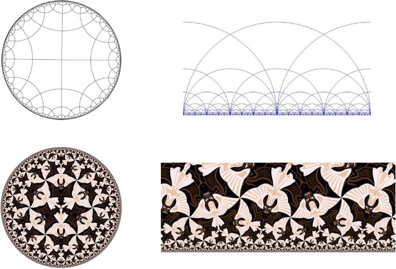
M. C. Escher’s “Circle Limit IV” © 2026 The M. C. Escher Company – The Netherlands. All rights reserved.
The hyperbolic structure in Alberto Burri’s Grande cretto nero
But what about the cracks themselves? At the Centre Pompidou in Paris, among some of the most iconic artworks of the 20th century, one encounters a monumental black canvas by the Italian artist Alberto Burri1https://www.centrepompidou.fr/fr/ressources/personne/cbq6bAe (1915–1995): The Grande cretto nero (1977). This rectangular work, measuring 1.5 by 2.5 meters, is covered with a dense mosaic of fractures. The cracks are sharply defined, spreading across the entire surface. As the eye moves toward the edges, the fractured regions become smaller and smaller, similar to the shrinking tiles in Poincaré’s hyperbolic models.
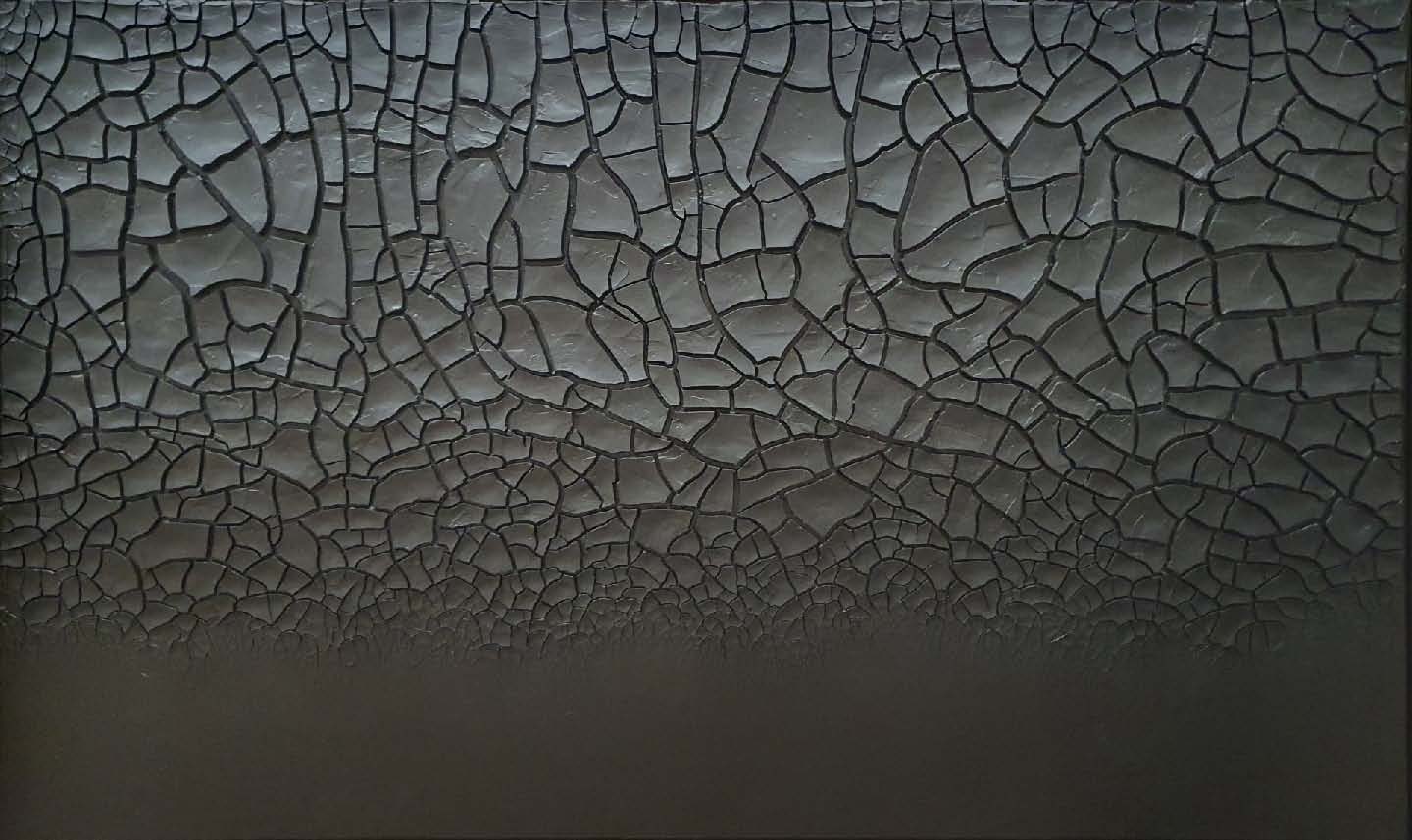
All rights reserved (© Alberto Burri / VG Bild-Kunst, Bonn 2026; Photo: bpk / MNAM-CCI, Dist. GrandPalaisRmn / Bertrand Prévost).
This hyperbolic flavor is especially evident at the lower boundary. The fragments visibly diminish in size as they approach the edge, while the cracks themselves often follow curved lines that meet the boundary at right angles, just like geodesics in Poincaré’s upper half-plane. At first this may seem puzzling, but it becomes less surprising if we recall what was said earlier about cracks: they naturally seek to release stress by meeting boundaries or other cracks at angles close to 90°. In Burri’s work, the cracks formed near the edges follow precisely this principle, bending in ways that maximize the release of tension as they approach the boundary. The same kind of hyperbolic behavior can sometimes be observed in the cracked surfaces of old roads and pavements.
Seen this way, Burri’s work brings to mind Poincaré’s upper half-plane, especially along the lower edge where the fragments shrink, and the cracks meet the boundary at right angles. Yet unlike the half-plane, which is bounded only from below, Burri’s rectangular canvas is enclosed on all four sides, and a similar hyperbolic behavior emerges along every edge. This brings the analogy even closer to Poincaré’s disc model, where space contracts uniformly toward all boundaries. It is therefore natural to ask how Burri’s cretto would look like if reimagined within a disc?
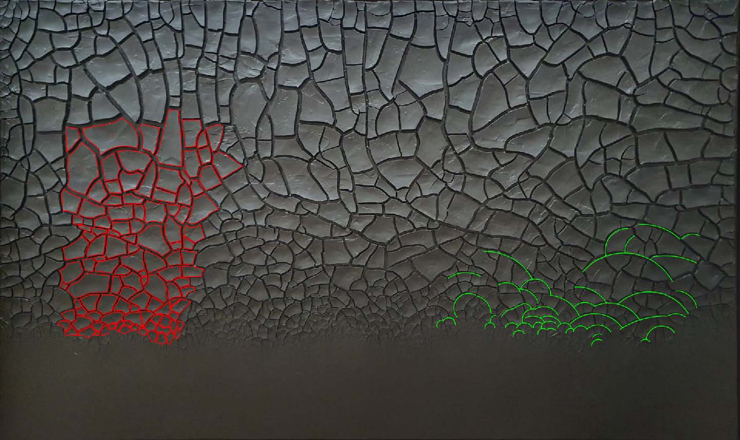
All rights reserved (© Alberto Burri / VG Bild-Kunst, Bonn 2026; Photo: MNAM-CCI, Dist. GrandPalaisRmn / Bertrand Prévost)
Mapping the square to the disc
Poincaré’s upper half-plane and the disc are equivalent models of hyperbolic space, connected by transformations that preserve their geometry. Burri’s canvas, however, is a rectangle so that these standard transformations do not readily apply. To preserve the crucial behavior of the cracks meeting at right angles (especially at the boundary), we require a transformation that preserves angles, a so-called conformal transformation. Fortunately, there is such a transformation which does exactly what we need: the Schwarz–Christoffel transformation.
More precisely, the Schwarz–Christoffel (SC) transformation provides a conformal map between the unit disc
and polygonal regions of the plane. In the case of a square, explicit formulas can even be written down using elliptic integrals. Following Fong [2 C. Fong, The conformal hyperbolic square and its ilk. In: Proceedings of Bridges 2016: Mathematics, Music, Art, Architecture, Education, Culture. pp. 179–186 (2016) ], the forward map
from the disc to the square is given by
where is the incomplete Legendre elliptic integral of the first kind with modulus , and is the complete elliptic integral of the first kind. Explicitly,
Computational implementation
To actually use the Schwarz–Christoffel transformation to map Burri’s work to a disc, we wrote a Python program that constructs the image in the disc pixel by pixel. The procedure can be summarized as follows:
Load and center-crop the source image to a square domain.
Construct a uniform Cartesian grid in the unit disc.
For each disc point , compute its image in the square.
Convert into pixel coordinates and assign to the corresponding color from the square image.
Assemble all pixels to obtain the disc-shaped image.
Reinterpreting Burri’s Grande cretto nero as a disc
The implementation we described above sends a square image conformally onto the disc. However, Burri’s Grande cretto nero is rectangular rather than square. A direct mapping of the rectangle to the disc would inevitably produce horizontal squeezing and distortions, obscuring the geometric features we wish to preserve.
To avoid this, we first reinterpret Burri’s canvas as a square. Concretely, we crop out the central region of the painting and conceptually “glue” its left and right parts together to form a square image. This step sacrifices the rectangular proportions but preserves the essential crack structure at the boundaries.
Once reinterpreted as a square, the image can be conformally mapped onto the unit disc. The crack geometry is faithfully preserved: fractures remain orthogonal to the boundary, while the overall structure acquires the characteristic hyperbolic flavor familiar from Poincaré’s disc model. Beyond this, the resulting image strikingly evokes the hyperbolic patterns of Escher’s Circle Limit I–IV. Yet there is a crucial difference: Escher’s artworks are deliberate drawings, where he intentionally depicts hyperbolic geometry, whereas in Burri’s work, the structure arises spontaneously from cracks, purely shaped by physical laws.
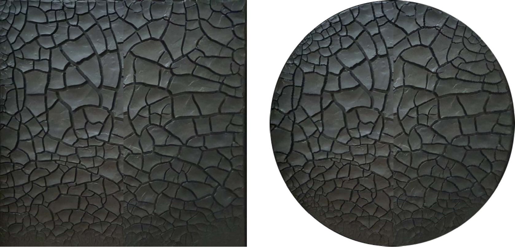
All rights reserved (© Alberto Burri / VG Bild-Kunst, Bonn 2026; Photo: MNAM-CCI, Dist. GrandPalaisRmn / Bertrand Prévost)
Some more hyperbolic art from the Grande cretto nero
Beyond simply removing the central region to obtain a square image of Grande cretto nero, alternative constructions are possible. One such approach consists in cropping specific triangular sections from the artwork and assembling copies of them to form a square. This procedure introduces artificial symmetries which may be perceived as visually appealing. However, they depart from the purely natural crack formation that characterizes Burri’s original composition, as illustrated in our earlier example (Figure 12). Below, we present several instances obtained from different triangular selections.
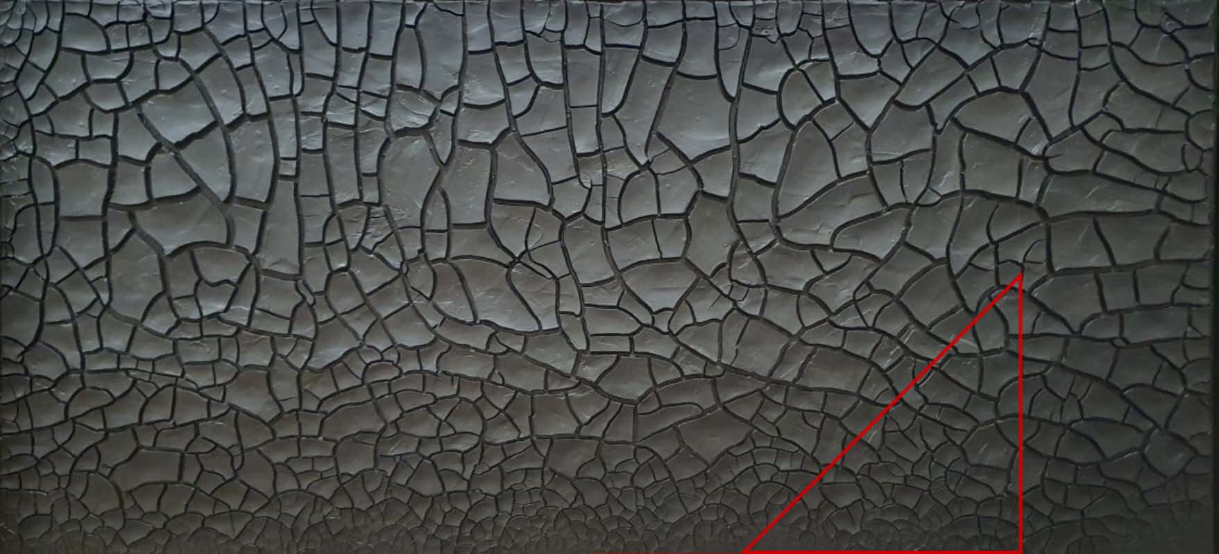
All rights reserved (© Alberto Burri / VG Bild-Kunst, Bonn 2026; Photo: MNAM-CCI, Dist. GrandPalaisRmn / Bertrand Prévost)
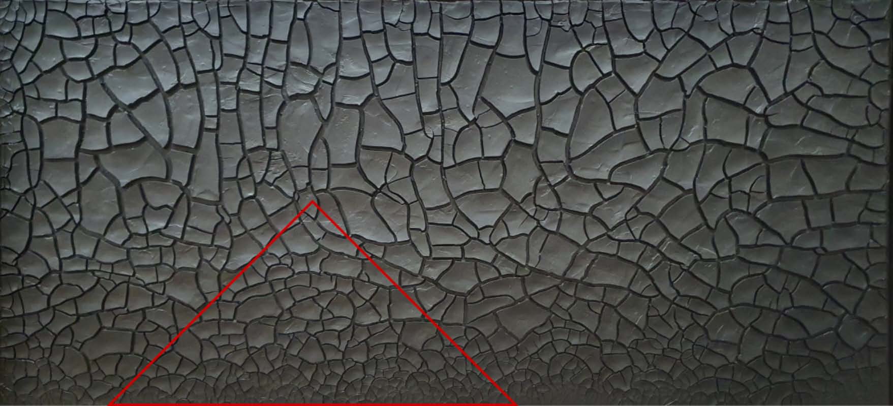
All rights reserved (© Alberto Burri / VG Bild-Kunst, Bonn 2026; Photo: MNAM-CCI, Dist. GrandPalaisRmn / Bertrand Prévost)
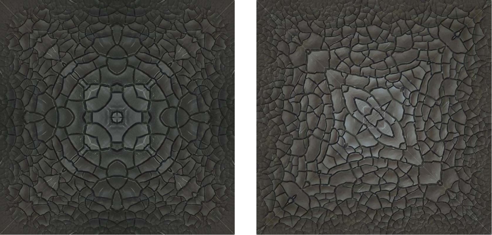
All rights reserved (© Alberto Burri / VG Bild-Kunst, Bonn 2026; Photo: MNAM-CCI, Dist. GrandPalaisRmn / Bertrand Prévost)
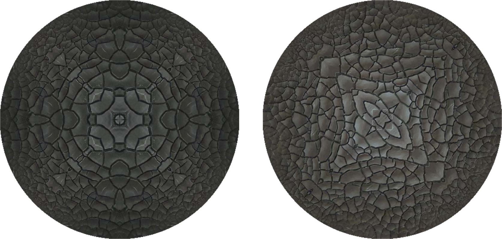
All rights reserved (© Alberto Burri / VG Bild-Kunst, Bonn 2026; Photo: MNAM-CCI, Dist. GrandPalaisRmn / Bertrand Prévost)
An invitation to the unintentional
From simple mud cracks to traces of life on Mars to hyperbolic structures in art: what may at first seem like a trivial observation, a simple curiosity, can grow into a more profound inquiry that opens unexpected connections. Careful attention reveals structures that link, in our case, material science, physics, and mathematics, and at times even unexpectedly resonate with art. At these crossings, disciplines merge with one another, leaving behind ties deeper than any single field alone.
I therefore invite you to stay curious, to pause and take time for the “little things,” the unexpected and the unintentional. For it is precisely in these moments that familiar knowledge often expands into new insights.
Python implementation of the Schwarz–Christoffel mapping transformation
Python code implementing the Schwarz–Christoffel transformation to map a square image conformally onto a disc. This code was used to generate the disc versions of Burri’s Grande cretto nero.
import numpy as np from PIL import Image from mpmath import ellipf import cmath
# -- User settings -- INPUT_PATH = "input.png" # square input image OUTPUT_PATH = "output_disc.png" RES = 512 # output resolution (diameter)
# -- Load and square-crop input -- im = Image.open(INPUT_PATH).convert("RGB") W, H = im.size side = min(W, H) left = (W - side) // 2 top = (H - side) // 2 im_sq = im.crop((left, top, left+side, top+side)) src = np.asarray(im_sq) S = side
# -- Constants -- Ke = 1.8540746773013719184 # complete elliptic integral K(m=1/2) m_param = 0.5 one_over_sqrt2 = 1.0 / np.sqrt(2.0)
# -- Output grid on unit disc -- x = np.linspace(-1, 1, RES) y = np.linspace(-1, 1, RES) X, Y = np.meshgrid(x, y) R = np.sqrt(X*X + Y*Y) mask = R <= 1.0 out = np.ones((RES, RES, 3), dtype=np.uint8) * 255
def z_to_src_xy(z): zx, zy = np.real(z), np.imag(z) px = (zx + 1.0) * 0.5 * (S - 1) py = (zy + 1.0) * 0.5 * (S - 1) return int(np.clip(round(px), 0, S-1)), int(np.clip(round(py), 0,S-1))
# -- Schwarz–Christoffel map -- for iy in range(RES): for ix in range(RES): if not mask[iy, ix]: continue w = complex(X[iy, ix], Y[iy, ix]) phi = cmath.acos((1.0+1.0j) * w * one_over_sqrt2) Fphi = ellipf(phi, m_param) z = ((1.0-1.0j)/(-Ke)) * Fphi + (1.0-1.0j) jx, jy = z_to_src_xy(z) out[iy, ix] = src[jy, jx]
Image.fromarray(out).save(OUTPUT_PATH) print(f"Saved OUTPUT_PATH")
Copyright disclaimer
Creative Commons license terms for re-use do not apply to the pictures in this article and further permission may be required from the right holder.
References
- G. Domokos, D. J. Jerolmack, F. Kun and J. Török, Plato’s cube and the natural geometry of fragmentation. Proc. Natl. Acad. Sci. USA 117, 18178–18185 (2020)
- C. Fong, The conformal hyperbolic square and its ilk. In: Proceedings of Bridges 2016: Mathematics, Music, Art, Architecture, Education, Culture. pp. 179–186 (2016)
- W. Rapin, G. Dromart, B. C. Clark, J., Schieber, E. S. Kite, L. C. Kah, L. M. Thompson, O. Gasnault, J. Lasue, P.-Y. Meslin, P. I. Gasda and N. L. Lanza, Sustained wet–dry cycling on early Mars. Nature 620, 299–302 (2023)
Cite this article
Julien Meyer, The hidden art in things breaking apart. Eur. Math. Soc. Mag. 139 (2026), pp. 19–25
DOI 10.4171/MAG/303